Macro view of NMR

Magnetism instead of transitions

NMR at the level of the sample rather than the nucleus requires a complete change of thinking and a lot of math. The focus on the main page will be the thinking part, the math can be accessed on separate pages via links. The instrument utilizes magnetic induction rather than photon absorption. A transmitter causes changes in the magnetic fields of a sample, which then induce currents in a detector coil which are picked up by a receiver. So understanding NMR at a macro level requires intimate knowledge of magnetic moments and induction.

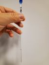
First the sample has to be defined. Ethanol is a good starting sample for analysis. It is a simple molecule, a liquid at room temperature with good flow rate (low viscosity) and slow evaporation rate (low vapor pressure). The molecule has 6 hydrogens, 2 carbons and an oxygen (CH₃CH₂OH), and there is not much self-association at room temperature. The sample container will be a 5mm glass tube:

About 0.75ml of ethanol in the tube will make a perfect sample for introduction to NMR.

All matter that is charged also has a magnetic field. Why? Good luck with that. Technically, if a charge isn't moving it isn't supposed to have a magnetic field, but since movement is relative, everything is moving compared to something else, so everything that is charged has a magnetic field. At any rate, since every atom has positively charged protons in the nucleus and negatively charged electrons surrounding the nucleus, there should be a net magnetic field around each atom. Similarly, there should be a net magnetic field around every molecule since the atoms are bonded to each other via electrons which all have charge and thus magnetic fields. However, a complication to this picture is that atoms and electrons also have a property called spin, and this property affects an atom's net magnetic field, and thus whether there is an actual net magnetic field.

It turns out that the main ¹H isotope of hydrogen (called proton in the NMR literature) and the ¹³C isotope of carbon (called carbon in the NMR literature) have net magnetic fields while the main isotope of oxygen and the main ¹²C isomer of carbon do not.

In summary, in the NMR tube of ethanol there is a solution of tiny bar magnets of ¹H and ¹³C.

On the benchtop, the bar magnets floating around in solution are randomly oriented, so the bar magnets average out. If placed into a strong magnetic field however, some of the floating bar magnets will line up with the field, generating a net magnetic field for each ¹H and ¹³C. If magnetism was the only factor then the floating bar magnets would line up with the external field and that would be it, nothing more would happen. The key part about NMR is that these magnets are also spinning, so there is torque that causes a precession around the axis of the external field. This precession frequency is what is probed with a transmitter.

Spectra vs Transition Spectra

To obtain a spectrum, the sample is placed into a static magnetic field to cause alignment of the magnets within a sample and their precession about the external magnetic field axis. This frequency depends on the gyromagnetic ratio (gamma) (g) for that element/elementary particle (a constant) and the intensity of the static magnetic field (B₀) according to the derived equation:

v₀=g*B₀

Since this v₀ is a moving charge, this represents electromagnetic frequency and can interact with an external electromagnetic frequency according to the usual rules of wave mechanics. In short, if an external electromagnetic frequency of the same magnitude is applied to the sample, it can 'resonate' with the sample, depending on the phases of the two fields. Fortunately, the gyromagnetic ratios of components of a sample are dramatically different, so a transmitter/receiver pair can be set up to 'look' at just one of the many v₀ in a sample.

Based on the Larmor equation, the only variable for a particular atomic component is the external field strength B₀, but since there are magnetic fields all around a molecule of the sample, each atomic component will experience slightly different B, and thus have slightly different v. Thus the transmitter/receiver pair will see several resonances for each atomic component in a sample of a molecule such as ethanol and it is these resonances that are studied in NMR. In addition, the atoms in a molecule that are in the same magnetic environment will experience the same B and thus have the same v and give the same peak.

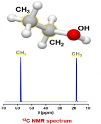
For the sample of ethanol there are three groups of protons, and two groups of carbons, so there should be 3 peaks in the proton spectrum and 2 peaks in the carbon spectrum (the splitting in the proton spectrum and lack of splitting in the carbon spectrum will be discussed later):

For both spectra the x axis is relative frequency while the y axis is relative intensity.

Radio Pulse Power vs Transition Pulse Power

Radio pulse power is where the macro view of NMR changes dramatically from micro view. The situation at the start of an experiment is the sample suspended in a strong magnetic field so any net magnetic dipoles start precessing around the external magnetic field axis.

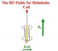
Then a transmitter in an axis orthogonal to the main magnetic field (B₀) sends an Rf pulse, which creates a new magnetic field called B₁:

Since the dipole magnet is precessing, it is common to look at the Z-component of the dipole magnet vector, called M₀.The new magnetic field B₁ pulls the net dipole down into the XY plane, and since the Rf is oscillating the new magnetic field B₁ cycles plus and minus and will cause the dipole to push all the way to -Z and back up to +Z again, depending on how long the Rf pulse is. Once the transmitter is turned off the receiver is turned on and as the dipole relaxes back to +Z again, the moving magnet induces a current in the receiver coil which is picked up as a signal in the detector.

Image of pulse on dipoles. In this image the detector only picks up magnetization along the X axis, so when the dipole magnet vector goes to + or - Z, the signal goes to 0.

Since the receiver is along the X axis, the pulse power to give the strongest signal is the one that pulls the net dipole down completely into the XY plane. This amount of pulse is called the 90 degree pulse, since it pulls the dipole 90 degrees from the Z axis. Pulse power is watts times time, and the watts is constant so the time is varied, with the resulting pulses given in microseconds. It is normal for the watts to be set such that the 90 degree pulse is between 5 and 10 microseconds.